
In today’s fast-changing world, the cyber threat landscape is getting increasingly complex and signature-based systems are falling behind to protect endpoints. All major security solutions are built with layered security models to protect endpoints from today’s advanced threats. Machine learning-based detection is also becoming an inevitable component of these layered security models. In this post, we are going to discuss how Quick Heal is incorporating machine learning (ML) in its products to protect endpoints.
Use of ML or AI (artificial intelligence) has already been embraced by the security industry. We, at Quick Heal, are using ML for different use cases. One of them is an initial layer of our multi-level defense. The main objective of this layer is to determine the suspiciousness of a given file or sample. If it finds the file as suspicious, then the file will be scrutinized with the next layers. This filtering reduces the load on the other security layers.
Here, we are going to discuss how we use static analysis of PE files using ML to filter out the traffic sent to the next security layers.
Machine learning overview
In machine learning, we try to give computers the ability to learn from data instead of programmed explicitly. In our problem statement, we can use the power of ML to make a model that is trained on the known data of clean and malicious files and that can further predict the nature of unknown sample files. The key requirement for building ML models is to have data for training. And it must be accurately labeled otherwise results and predictions can be misleading.
The process starts with organizing a trained set by collecting a large number of clean and malicious samples and labeling them. We extract features from these samples (for our models we extracted features from PE headers of all the collected samples). Then the model is trained by providing these feature matrices to it – as shown in the block diagram below.
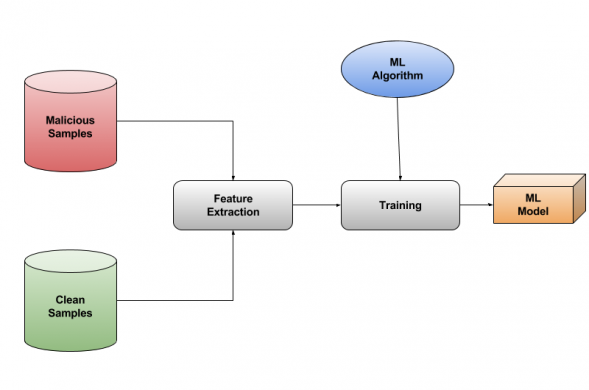
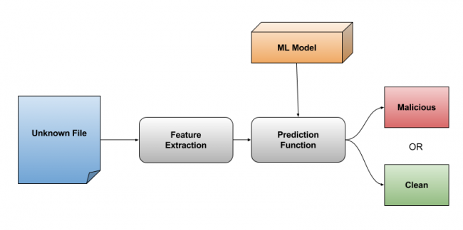
A feature array of an unknown sample is provided to this trained model. It returns a confidence score for that sample suggesting whether this file is similar to a clean or malicious set.
Feature selection
A feature is an individual measurable property or characteristic of the things being observed. For example, if we want to classify cats and dogs we can take features like “type of fur”, “loves the company of others or loves to stay alone”, “barks or not”, “number of legs”, “very sharp claws”, etc.
Selecting good features is one of the most important steps in training any ML model. As shown in the above example, if we select “number of legs” as a feature for training, it won’t be possible to classify that both dogs and cats have the same number of legs. But, if we take “bark or not”, it would be a good classifier as dogs bark and cats don’t. Also “sharpness of claws” would be a good feature.
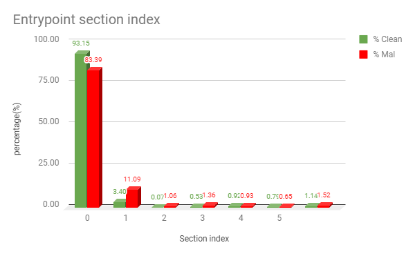
On similar lines, to classify malicious samples from clean ones, we need to have features. So, we start with deriving pe file header attributes which need fewer computations to extract. We have some Boolean kind features like “EntryPoint present in First Section”, “Resource present” or “Section has a special character in its name”. And some count or value-based like “NumberOfSections”, “File TimeDateStamp”, etc. Some of these features are so strong that many times they act as good separator for malicious and benign samples. We will try to explain this by following two examples. As shown in the following graph 1.0, in most of the cases, for clean files, the entry point section is the 0th section, but for malicious files, it may vary.
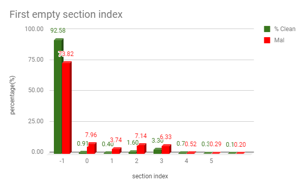
Similarly, for an index of “First empty section” of a file, we get the following plot.
Feature scaling
The data we feed to our model must be scaled properly. For example, the value of attribute like Address_OF_EntryPoint = 307584 will have a very large value when compared with the value of attribute like No_Of_Sections = 5. Such a huge difference can cause our model to be poorly trained. We use min_max scaling to scale the data. Here, we bring all the features to the same range in this case 0 to 1.
Dimensionality reduction
The next step is dimensionality reduction. In data, many times there are groups of features that are co-related to each other, i.e. if one feature changes, others also change at some rate. Removing or combining such features saves space and time and improves the performance of machine learning models. This process of reducing the number of unwanted or redundant features is known as dimensionality reduction. This ensures models are trained and tested faster without compromising the accuracy. We tried using PCA (Principal Component Analysis), Select K-Best by various algorithms.
PCA is used to convert a set of observations of possibly correlated variables into a set of values of linearly uncorrelated variables called principal components. PCA tries to find the principal components so as the distance between our samples and the principal component is minimized. The lesser is the distance between samples and principal components, the more variance is retained.
We can make a plot of cumulative variance versus the number of principal components to find the number of Principal Components (PCs) required to cover almost all data. Applying PCA on our data and tuning it gives us 163 PCs for nearly 1000 different features. That means now we can train the model on 163 features that can almost cover the complete data set.
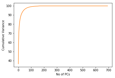
We can transform our test data into these 163 Principal Components and can apply classification models. Though PCA works fine, we need to calculate PCs at a client’s end before prediction. So, we settled with Select K-Best using Chi-squared statistics, which gives k number of best features by finding out their importance after comparing whole data.
Training
The next step is about training the model. While training, we need to focus on the following parameters:
Size of Model: The model generated by any algorithm should have an optimal size and updating it should take minimal of efforts.
Training Time: Time and resources utilized by an algorithm while training should be minimal (though it is not a primary requirement).
Prediction Time: Prediction function must be as fast as possible.
Overfitting: Some algorithms work great on small datasets. But, as we grow the dataset the results tend to go down this is called overfitting.
We tried a few algorithms; Logistic Regression worked good on small datasets but it tends to overfit & the accuracy reduces as we increase the training set.
Then we tried Random Forest Classifier. Accuracy here is good but the size of the model that is generated is large as it is a forest of multiple decision trees. And prediction function also takes time as trees need to be traversed. So we moved to SVM (Support Vector Machine).
Support vector machines
Support vector machine (SVM) is a supervised machine learning algorithm which can be used for both classification and regression challenges. However, it is mostly used in classification problems. In this algorithm, we plot each data item as a point in n-dimensional space (where n is a count of features you have) with the value of each feature being the value of a particular coordinate. Then, we perform a classification by finding the hyperplane that differentiates the two classes properly.
There can be a lot of hyperplanes classifying the data, but SVM targets to find out a hyperplane that has the largest distance from the nearest sample set on both sides of the plane.
For example, here SVM will choose plane C, among A and B.
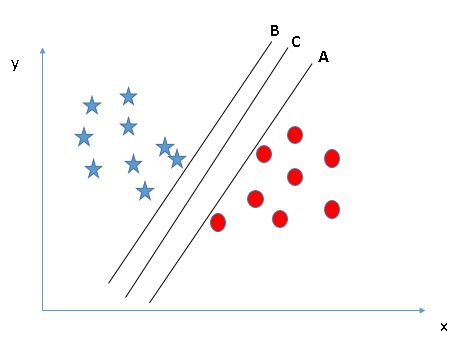
The example above is of Linear SVM. By using kernel functions in SVM, we can classify non linearly distributed data as well. The kernel function is a function which takes two inputs and outputs a number representing how similar they are. Generally used kernels in SVM are Linear kernel, Polynomial kernel, Radial bias function kernel (RBF). We tried with all of these kernels and found that RBF and Linear work well for our data. As linear kernel has an extremely fast prediction function, we finalized it. The prediction function is (w*x + b) where w is a vector of support vectors, x is a feature vector of the test sample and b is intercept or bais.
The SVM model trained using the above steps has a very good accuracy that it nearly reduced 1/3rd of the traffic to next levels. It is helping us greatly in improving performance and accuracy of detection.
Conclusion
Machine learning can be effectively used by the antivirus industry and use cases are huge. Quick Heal is committed to bringing the latest research in ML to reform endpoint security. At Quick Heal, we practice ML at various stages and the above case study is one of them. In the future, we will share write-ups on other case studies.